Bulk matter — the D track

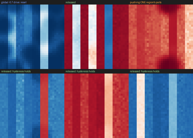
One field per cell, updated as new x = tanh(J·(neighbour mix) + region bias + input field − fatigue·a) + noise. When the coupling J exceeds ~1.15, agreement between neighbours becomes self-reinforcing and whole regions lock into the same sign: the grid stops acting like independent cells and starts acting like a material. The grid is cut into vertical stripes (regions) with no neighbour links across boundaries — each stripe is its own quasi-independent magnet. Higher worlds add per-region response speeds (some react in ~20 ticks, some 25× slower) and a slow fatigue variable that integrates recent activation and pushes back — hold a region "up" too long and it rebounds, even oscillates, after release. The discoverable laws are collective: switching thresholds, hysteresis, relaxation schedules, fatigue rebound.

← all tracks & how the worlds work

D0 — 1 module(s), 6 inputs / 24 sensors (0 dead)

Clean senses, one collective mode. 6 inputs, 24 well-behaved sensors, low noise. The tutorial world: find polarities, find the switch, map the loop.

lattice 24×24 · coupling J=1.35 · micro noise σ=0.04 · sensor noise 0.02 · sign-flip prob 0.0 · tick budget 80,000

port wiring
micro lattice snapshots
hysteresis loops
agent-view time series

D1 — 1 module(s), 6 inputs / 32 sensors (4 dead)

Same law, murky senses: 4 dead channels, 35% inverted sensors, gain spread 0.6–1.6×, more noise. Tests sensor calibration before science.

lattice 24×24 · coupling J=1.35 · micro noise σ=0.05 · sensor noise 0.05 · sign-flip prob 0.35 · tick budget 80,000

port wiring
micro lattice snapshots
hysteresis loops
agent-view time series

D2 — 3 module(s), 6 inputs / 36 sensors (4 dead)

Three semi-independent regions (modules) with their own switches + murky senses. Local inputs matter: which port drives which region?

lattice 24×24 · coupling J=1.35 · micro noise σ=0.05 · sensor noise 0.05 · sign-flip prob 0.35 · tick budget 100,000

port wiring
micro lattice snapshots
hysteresis loops
agent-view time series

D3 — 6 module(s), 8 inputs / 48 sensors (8 dead)

Six modules, weak global coupling, tighter budget. Requires targeted per-region experiments and bookkeeping.

lattice 30×30 · coupling J=1.45 · micro noise σ=0.06 · sensor noise 0.07 · sign-flip prob 0.4 · tick budget 60,000

port wiring
micro lattice snapshots
hysteresis loops
agent-view time series

D4 — 8 module(s), 10 inputs / 60 sensors (10 dead)

Frontier: 8 modules, per-module response speeds (25× spread), and a slow fatigue variable (~200-tick memory) that turns the world into a slow relaxation oscillator. Duration of drive matters; states drift for hundreds of ticks after release. Best current agents: ~0.2–0.4.

lattice 32×32 · coupling J=1.4 · micro noise σ=0.06 · sensor noise 0.08 · sign-flip prob 0.4 · tick budget 150,000

port wiring
micro lattice snapshots
hysteresis loops
agent-view time series
adaptation dynamics
FILM (god view, D4): a global −0.7 drive resets every region down; pushing the ports of ONE region flips just that stripe; after release, hysteresis holds the flip while fatigue slowly pushes back. This memory-with-rebound is the physics the S1 stratum probes — the one every frontier model still fails.

Generated by python -m physim.viz from the real engine (seed 0 of each preset). God-view panels and films use evaluator-only accessors; agent-view panels use only the public interface. How scoring works.